14  Performance

This chapter explains simple options and settings to improve the efficiency of your targets pipelines. It also explains how to monitor the progress of a pipeline currently running.¹

Summary: efficiency

Basic efficiency:

• Storage: choose efficient data storage formats for targets with large data output.
• Memory: consider memory = "transient" and the garbage_collection option for high-memory tasks.
• Overhead: if each task runs quickly, batch the workload into smaller numbers of targets to reduce overhead.

Parallel processing:

• Distributed computing: consider distributed computing with crew.
• Worker storage: parallelize the data processing with storage = "worker" and retrieval = "worker".
• Local targets: consider deployment = "main" for quick targets that do not need parallel workers.

Esoteric optimizations:

• Metadata: set seconds_meta_append, seconds_meta_upload, and seconds_reporter to be kind to the local file system and R console.
• Timestamps: Set trust_timestamps = TRUE to avoid recomputing hashes of targets that are already up to date.

Summary: monitoring

• targets has functions like tar_progress() and tar_watch() to monitor the progress of the pipeline.
• Profiling with the proffer package can help discover bottlenecks.

14.1 Basic efficiency

These basic tips help most pipelines run efficiently.

14.1.1 Storage

The default data storage format is RDS, which can be slow and bulky for large data. For large data pipelines, consider alternative formats to more efficiently store and manage your data. Set the storage format using tar_option_set() or tar_target():

tar_option_set(format = "qs")

Tips about data formats

Some formats such as "qs" work on all kinds of data, whereas others like "feather" works only on data frames. Most non-default formats store the data faster and in smaller files than the default "rds" format, but they require extra packages to be installed. For example, format = "qs" requires the qs package, and format = "feather" requires the arrow package.

For extremely large datasets that cannot fit into memory, consider format = "file" to treat the data as a file on disk. Downstream targets are free to load only the subsets of the data they need.

14.1.2 Memory

targets makes decisions about how long to keep target results in memory and when to run garbage collection. You can customize this behavior with the memory and garbage_collection arguments of tar_option_set().²

tar_option_set(
  memory = "transient",
  garbage_collection = 10 # Can be an integer in version >= 1.8.9003
)

These arguments are available to tar_target() as well, although garbage_collection is a TRUE/FALSE value indicating whether to run garbage collection to run just before that specific target runs.

tar_target(
  name = example_data,
  command = get_data(),
  memory = "transient"
  garbage_collection = TRUE
)

About memory and garbage collection

memory = "transient" tells targets to remove data from the R environment as soon as it is no longer needed. However, the computer memory itself is not freed until garbage collection is run, and even then, R may not decrease the size of its heap. You can run garbage collection yourself with the gc() function in R.

Transient memory and garbage collection have tradeoffs: the pipeline reads data from storage far more often, and these data reads take additional time. In addition, garbage collection is usually a slow operation, and repeated garbage collections could slow down even a small pipeline with a mere thousand targets.

garbage_collection = 100 tells targets to run gc() every 100th active target, both locally and on each parallel worker. The default value is 1000 if not specified directly.

14.2 Overhead

Each target incurs overhead, and it is not good practice to create millions of targets which each run quickly. Instead, consider grouping the same amount of work into a smaller number of targets. See the sections on what a target should do and how much a target should do.

About batching

Simulation studies and other iterative stochastic pipelines may need to run hundreds of thousands of independent random replications. For these pipelines, consider batching to reduce the number of targets while preserving the number of replications. In batching, each batch is a dynamic branch target that performs a subset of the replications. For 1000 replications, you might want 40 batches of 25 replications each, 10 batches with 100 replications each, or a different balance depending on the use case. Functions tarchetypes::tar_rep(), tarchetypes::tar_map_rep(), and stantargets::tar_stan_mcmc_rep_summary() are examples of target factories that set up the batching structure without needing to understand dynamic branching.

14.3 Parallel processing

These tips add parallel processing to your pipeline and help you use it effectively.

14.3.1 Distributed computing

Consider distributed computing with crew, as explained at https://books.ropensci.org/targets/crew.html. The targets package knows how to run independent tasks in parallel and wait for tasks that depend on upstream dependencies. crew supports backends such as crew.cluster for traditional clusters and crew.aws.batch for AWS Batch.

14.3.2 Worker storage

If you run tar_make() with a crew controller, then parallel processes will run your targets, but the main R process still manages all the data by default. To delegate data management to the parallel crew workers, set the storage and retrieval settings in tar_target() or tar_option_set():

tar_option_set(storage = "worker", retrieval = "worker")

But be sure those workers have access to the data. They must either find the local data, or the targets must use cloud storage.

14.3.3 Local targets

In distributed computing with targets, not every target needs to run on a remote worker. For targets that run quickly and cheaply, consider setting deployment = "main" in tar_target() to run them on the main local process:

tar_target(dataset, get_dataset(), deployment = "main")
tar_target(summary, compute_summary_statistics(), deployment = "main")

14.4 Monitoring progress

Even the most efficient targets pipelines can take time to complete because the user-defined tasks themselves are slow. There are convenient ways to monitor the progress of a running pipeline:

1. tar_poll() continuously refreshes a text summary of runtime progress in the R console. Run it in a new R session at the project root directory. (Only supported in targets version 0.3.1.9000 and higher.)
2. tar_visnetwork(), tar_progress_summary(), tar_progress_branches(), and tar_progress() show runtime information at a single moment in time.
3. tar_watch() launches an Shiny app that automatically refreshes the graph every few seconds.

Example: monitoring the pipeline with tar_watch()

# Define an example target script file with a slow pipeline.
library(targets)
library(tarchetypes)
tar_script({
  sleep_run <- function(...) {
    Sys.sleep(10)
  }
  list(
    tar_target(settings, sleep_run()),
    tar_target(data1, sleep_run(settings)),
    tar_target(data2, sleep_run(settings)),
    tar_target(data3, sleep_run(settings)),
    tar_target(model1, sleep_run(data1)),
    tar_target(model2, sleep_run(data2)),
    tar_target(model3, sleep_run(data3)),
    tar_target(figure1, sleep_run(model1)),
    tar_target(figure2, sleep_run(model2)),
    tar_target(figure3, sleep_run(model3)),
    tar_target(conclusions, sleep_run(c(figure1, figure2, figure3)))
  )
})

# Launch the app in a background process.
# You may need to refresh the browser if the app is slow to start.
# The graph automatically refreshes every 10 seconds
tar_watch(seconds = 10, outdated = FALSE, targets_only = TRUE)

# Now run the pipeline and watch the graph change.
px <- tar_make()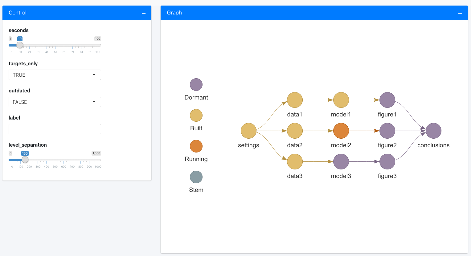

tar_watch_ui() and tar_watch_server() make this functionality available to other apps through a Shiny module.

14.5 Profiling

Profiling tools like profvis and proffer empirically identify the places where code runs slowly. It is important to identify these bottlenecks before you try to optimize. Visit https://r-prof.github.io/proffer/#why-use-a-profiler to see a motivating example of profiling in action.

To profile your project with profvis, run:

results <- profvis::profvis(
  targets::tar_make(
    callr_function = NULL, # Do not run the pipline behind a callr::r() process.
    use_crew = FALSE, # Disable parallel computing with crew (optional)
    as_job = FALSE # Do not run the pipeline in a Posit Workbench / RStudio background job.
  )
)
print(results, aggregate = TRUE) # aggregate = TRUE is crucial for interpretable flame graphs.

With proffer, profiling is similar.

proffer::pprof(
  targets::tar_make(
    callr_function = NULL, # Do not run the pipline behind a callr::r() process.
    use_crew = FALSE, # Disable parallel computing with crew (optional)
    as_job = FALSE # Do not run the pipeline in a Posit Workbench / RStudio background job.
  )
)

Poth packages render flame graphs that show where bottlenecks occur.

14.6 Resource usage

The autometric package can monitor the CPU and memory consumption of the various processes in a targets pipeline. This is mainly useful for high-performance computing workloads with parallel workers. Please read https://wlandau.github.io/crew/articles/logging.html for details and examples.

---

1. cue = tar_cue(file = FALSE) is no longer recommended for cloud storage. This unwise shortcut is no longer necessary, as of https://github.com/ropensci/targets/pull/1181 (targets version >= 1.3.2.9003).

2. As of version 1.8.0.9011, the default behavior of tar_make() (encoded with memory = "auto") is to release dynamic branches as soon as possible and keeps other targets in memory until the pipeline is finished. In addition, in targets >= 1.8.0.9003, the garbage_collection option can be a non-negative integer to control how often garbage collection happens (e.g. every 10th target).