15  Dynamic branching

Performance

Branched pipelines can be computationally demanding. See the performance chapter for options, settings, and other choices to optimize and monitor large pipelines.

15.1 Branching

Sometimes, a pipeline contains more targets than a user can comfortably type by hand. For projects with hundreds of thousands of targets, branching can make the code in _targets.R shorter and more concise.

targets supports two types of branching: dynamic branching and static branching. Some projects are better suited to dynamic branching, while others benefit more from static branching or a combination of both. Here is a short list of tradeoffs.

Dynamic	Static
Pipeline creates new targets at runtime.	All targets defined in advance.
Cryptic target names.	Friendly target names.
Scales to hundreds of thousands of branches.	Does not scale as easily, especially with tar_visnetwork() graphs
No metaprogramming required.	Familiarity with metaprogramming is helpful.

15.2 About dynamic branching

Dynamic branching is the act of defining new targets (called branches) while the pipeline is running (e.g. during tar_make()). Prior to launching the pipeline, the user does not need to know the number of branches or the input data of each branch.

To use dynamic branching, set the pattern argument of tar_target(). The pattern determines how dynamic branches are created and how the input data is partitioned among the branches. A branch is single iteration of the target’s command on a single piece of the input data. Branches are automatically created based on how the input data breaks into pieces, and targets automatically combines the output from all the branches when you reference the dynamic target as a whole.

15.3 Example

To illustrate, consider the example pipeline below. It uses dynamic branching to generate random spirographs using code borrowed from W. Joel Schneider’s spiro package.¹. A spirograph is a type of two-dimensional algebraic curve determined (in part) by parameters fixed_radius and cycling_radius. Targets fixed_radius and cycling_radius draw random parameter values, and the dynamic target points generates a spirograph dataset for each set of parameters (one spirograph per dynamic branch). Target single_plot plots each spirograph separately, and combine_plot plots all the spirographs together.

# _targets.R
library(ggplot2)
library(targets)
library(tarchetypes)
library(tibble)

# From https://github.com/wjschne/spiro/blob/87f73ec37ceb0a7a9d09856ada8ae28d587a2ebd/R/spirograph.R
# Adapted under the CC0 1.0 Universal license: https://github.com/wjschne/spiro/blob/87f73ec37ceb0a7a9d09856ada8ae28d587a2ebd/LICENSE.md
spirograph_points <- function(fixed_radius, cycling_radius) {
  t <- seq(1, 30 * pi, length.out = 1e4)
  diff <- (fixed_radius - cycling_radius)
  ratio <- diff / cycling_radius
  x <- diff * cos(t) + cos(t * ratio)
  y <- diff * sin(t) - sin(t * ratio)
  tibble(x = x, y = y, fixed_radius = fixed_radius, cycling_radius = cycling_radius)
}

plot_spirographs <- function(points) {
  label <- "fixed_radius = %s, cycling_radius = %s"
  points$parameters <- sprintf(label, points$fixed_radius, points$cycling_radius)
  ggplot(points) +
    geom_point(aes(x = x, y = y, color = parameters), size = 0.1) +
    facet_wrap(~parameters) +
    theme_gray(16) +
    guides(color = "none")
}

list(
  tar_target(fixed_radius, sample.int(n = 10, size = 2)),
  tar_target(cycling_radius, sample.int(n = 10, size = 2)),
  tar_target(
    points,
    spirograph_points(fixed_radius, cycling_radius),
    pattern = map(fixed_radius, cycling_radius)
  ),
  tar_target(
    single_plot,
    plot_spirographs(points),
    pattern = map(points),
    iteration = "list"
  ),
  tar_target(combined_plot, plot_spirographs(points))
)

tar_make()
#> + cycling_radius dispatched
#> ✔ cycling_radius completed [1ms, 50 B]
#> + fixed_radius dispatched
#> ✔ fixed_radius completed [0ms, 49 B]
#> + points declared [2 branches]
#> ✔ points completed [11ms, 309.30 kB]
#> + combined_plot dispatched
#> ✔ combined_plot completed [19ms, 1.69 MB]
#> + single_plot declared [2 branches]
#> ✔ single_plot completed [21ms, 1.81 MB]
#> ✔ ended pipeline [580ms, 7 completed, 0 skipped]

The final plot shows all the spirographs together.

tar_read(combined_plot)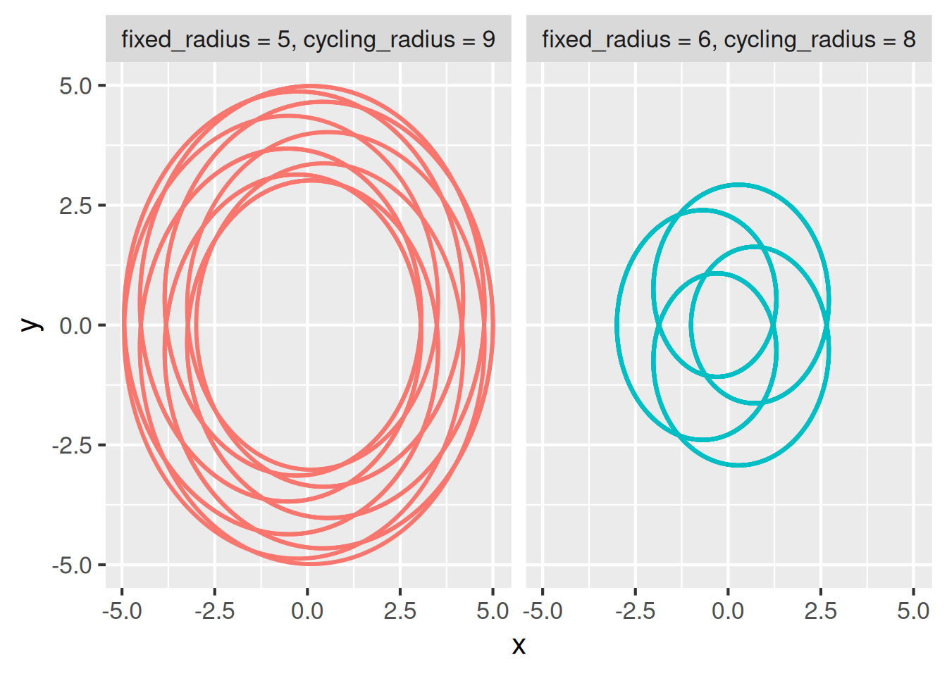

This plot comes from all the branches of points aggregated together. Because target points has iteration = "vector" in tar_target(), any reference to the whole target automatically aggregates the branches using vctrs::vec_c(). For data frames, this just binds all the rows.

tar_read(points)
#> # A tibble: 20,000 × 4
#>         x     y fixed_radius cycling_radius
#>     <dbl> <dbl>        <int>          <int>
#>  1 -1.26  -2.94            5              9
#>  2 -1.23  -2.95            5              9
#>  3 -1.20  -2.97            5              9
#>  4 -1.17  -2.98            5              9
#>  5 -1.14  -3.00            5              9
#>  6 -1.11  -3.01            5              9
#>  7 -1.08  -3.03            5              9
#>  8 -1.05  -3.04            5              9
#>  9 -1.02  -3.06            5              9
#> 10 -0.985 -3.07            5              9
#> # ℹ 19,990 more rows

By contrast, target single_plot list of branches because of iteration = "list".

tar_load(single_plot)
class(single_plot)
#> [1] "list"
length(single_plot)
#> [1] 2

Use the branches argument of tar_read() to read an individual branch or subset of branches.

tar_read(single_plot, branches = 1)
#> $single_plot_b415e3b98a99d41d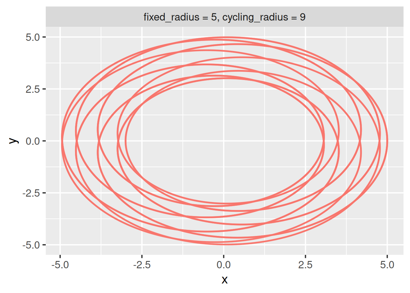

15.4 Provenance

Recall our dynamic target points with branches for spirograph datasets. Each branch has columns fixed_radius and cycling_radius so we know which parameter set each spirograph used. It is good practice to proactively append this metadata to each branch, e.g. in spirograph_points(). That way, if a branch errors out, it is easy to track down the upstream data that caused it.²

tar_read(points, branches = 1) # first branch
#> # A tibble: 10,000 × 4
#>         x     y fixed_radius cycling_radius
#>     <dbl> <dbl>        <int>          <int>
#>  1 -1.26  -2.94            5              9
#>  2 -1.23  -2.95            5              9
#>  3 -1.20  -2.97            5              9
#>  4 -1.17  -2.98            5              9
#>  5 -1.14  -3.00            5              9
#>  6 -1.11  -3.01            5              9
#>  7 -1.08  -3.03            5              9
#>  8 -1.05  -3.04            5              9
#>  9 -1.02  -3.06            5              9
#> 10 -0.985 -3.07            5              9
#> # ℹ 9,990 more rows

tar_read(points, branches = 2) # second branch
#> # A tibble: 10,000 × 4
#>           x     y fixed_radius cycling_radius
#>       <dbl> <dbl>        <int>          <int>
#>  1 -0.112   -1.44            6              8
#>  2 -0.0965  -1.44            6              8
#>  3 -0.0813  -1.45            6              8
#>  4 -0.0659  -1.46            6              8
#>  5 -0.0505  -1.47            6              8
#>  6 -0.0350  -1.47            6              8
#>  7 -0.0194  -1.48            6              8
#>  8 -0.00377 -1.49            6              8
#>  9  0.0120  -1.49            6              8
#> 10  0.0278  -1.50            6              8
#> # ℹ 9,990 more rows

15.5 Patterns

targets supports many more types of dynamic branching patterns.

• map(): one branch per tuple of elements.
• cross(): one branch per combination of elements.
• slice(): select individual pieces to branch over. For example, pattern = slice(x, index = c(3, 4)) branches over the third and fourth slices (or branches) of target x.
• head(): branch over the first few elements.
• tail(): branch over the last few elements.
• sample(): branch over a random subset of elements.

Patterns are composable. For example, pattern = cross(other_parameter, map(fixed_radius, cycling_radius)) is conceptually equivalent to tidyr::crossing(other_parameter, tidyr::nesting(fixed_radius, cycling_radius)). You can test and experiment with branching structures using tar_pattern(). In the output below, suffixes _1, _2, and _3, denote both dynamic branches and the slices of upstream data they branch over.

tar_pattern(
  cross(other_parameter, map(fixed_radius, cycling_radius)),
  other_parameter = 3,
  fixed_radius = 2,
  cycling_radius = 2
)
#> # A tibble: 6 × 3
#>   other_parameter   fixed_radius   cycling_radius  
#>   <chr>             <chr>          <chr>           
#> 1 other_parameter_1 fixed_radius_1 cycling_radius_1
#> 2 other_parameter_1 fixed_radius_2 cycling_radius_2
#> 3 other_parameter_2 fixed_radius_1 cycling_radius_1
#> 4 other_parameter_2 fixed_radius_2 cycling_radius_2
#> 5 other_parameter_3 fixed_radius_1 cycling_radius_1
#> 6 other_parameter_3 fixed_radius_2 cycling_radius_2

15.6 Iteration

The iteration argument of tar_target() determines how to split non-dynamic targets and how to aggregate dynamic ones. There are two major types of iteration: "vector" (default) and "list". There is also iteration = "group", which this chapter covers in the later section on branching over row groups.

15.6.1 Vector iteration

Vector iteration uses the vctrs package to intelligently split and combine dynamic branches based on the underlying type of the object. Branches of vectors are automatically vectors, branches of data frames are automatically data frames, aggregates of vectors are automatically vectors, and aggregates of data frames are automatically data frames. This consistency makes most data processing tasks extremely smooth.

Consider the following pipeline:

library(targets)
library(tarchetypes)
library(tibble)

list(
  tar_target(
    name = cycling_radius,
    command = c(1, 2),
    iteration = "vector"
  ),
  tar_target(
    name = points_template,
    command = tibble(x = c(1, 2), y = c(1, 2), fixed_radius = c(1, 2)),
    iteration = "vector"
  ),
  tar_target(
    name = points_branches,
    command = add_column(points_template, cycling_radius = cycling_radius),
    pattern = map(cycling_radius, points_template),
    iteration = "vector"
  ),
  tar_target(
    name = combined_points,
    command = points_branches
  )
)

tar_visnetwork()

tar_make()
#> + cycling_radius dispatched
#> ✔ cycling_radius completed [1ms, 53 B]
#> + points_template dispatched
#> ✔ points_template completed [2ms, 158 B]
#> + points_branches declared [2 branches]
#> ✔ points_branches completed [3ms, 336 B]
#> + combined_points dispatched
#> ✔ combined_points completed [0ms, 178 B]
#> ✔ ended pipeline [163ms, 5 completed, 0 skipped]

We observe the following:

tar_read(points_branches)
#> # A tibble: 2 × 4
#>       x     y fixed_radius cycling_radius
#>   <dbl> <dbl>        <dbl>          <dbl>
#> 1     1     1            1              3
#> 2     2     2            2              4

tar_read(points_branches, branches = 2)
#> # A tibble: 1 × 4
#>       x     y fixed_radius cycling_radius
#>   <dbl> <dbl>        <dbl>          <dbl>
#> 1     2     2            2              4

tar_read(combined_points)
#> # A tibble: 2 × 4
#>       x     y fixed_radius cycling_radius
#>   <dbl> <dbl>        <dbl>          <dbl>
#> 1     1     1            1              3
#> 2     2     2            2              4

iteration = "vector" produces convenient tibbles because:

1. vctrs::vec_slice() intelligently splits the non-dynamic targets for branching.
2. vctrs::vec_c() implicitly combines branches when you reference a dynamic target as a whole.

So the pipeline is equivalent to:

# cycling_radius target:
cycling_radius <- c(3, 4)

# points_template target:
points_template <- tibble(x = c(1, 2), y = c(1, 2), fixed_radius = c(1, 2))

# points_branches target:
points_branches <- lapply(
  X = seq_len(2),
  FUN = function(index) {
    # effect of iteration = "vector" in cycling_radius:
    branch_cycling_radius <- vctrs::vec_slice(cycling_radius, index)
    # effect of iteration = "vector" in points_template:
    branch_points_template <- vctrs::vec_slice(points_template, index)
    # command of points_branches target:
    add_column(branch_points_template, cycling_radius = branch_cycling_radius)
  }
)

# combined_points target:
points_branches$.name_spec = "{outer}_{inner}"
combined_points <- do.call( # effect of iteration = "vector" in points_branches
  what = vctrs::vec_c,
  args = points_branches
)

15.6.2 List iteration

iteration = "vector" does not know how to split or aggregate every data type. For example, vctrs cannot combine ggplot2 objects into a vector. iteration = "list" is a simple workaround that treats everything as a list during splitting and aggregation. Let’s demonstrate on a simple pipeline:

library(targets)
library(tarchetypes)
library(tibble)

list(
  tar_target(
    name = radius_origin,
    command = c(1, 2),
    iteration = "list"
  ),
  tar_target(
    name = radius_branches,
    command = radius_origin + 5,
    pattern = map(radius_origin),
    iteration = "list"
  ),
  tar_target(
    name = radius_combined,
    command = radius_branches
  )
)

tar_visnetwork()

tar_make()
#> + radius_origin dispatched
#> ✔ radius_origin completed [0ms, 53 B]
#> + radius_branches declared [2 branches]
#> ✔ radius_branches completed [0ms, 100 B]
#> + radius_combined dispatched
#> ✔ radius_combined completed [0ms, 137 B]
#> ✔ ended pipeline [150ms, 4 completed, 0 skipped]

We observe the following:

tar_read(radius_branches)
#> $radius_branches_a296b06d24ea0879
#> [1] 6
#> 
#> $radius_branches_5944b58b912631c4
#> [1] 7

tar_read(radius_branches, branches = 2)
#> $radius_branches_5944b58b912631c4
#> [1] 7

tar_read(radius_combined)
#> $radius_branches_a296b06d24ea0879
#> [1] 6
#> 
#> $radius_branches_5944b58b912631c4
#> [1] 7

As we see above, iteration = "list" uses [[ to split non-dynamic targets and list() to combine dynamic branches. Except for the special branch names above, our example pipeline is equivalent to:

# radius_origin target:
radius_origin <- c(1, 2)

# radius_branches target:
radius_branches <- lapply(
  X = seq_len(2),
  FUN = function(index) {
    # effect of iteration = "list" in radius_origin:
    branch_radius_origin <- radius_origin[[index]]
    # command of radius_branches:
    branch_radius_origin + 5
  }
)

# command of radius_combined:
radius_combined <- do.call( # effect of iteration = "list" in radius_branches
  what = list,
  args = radius_branches
)

15.7 Branching over row groups

To dynamically branch over dplyr::group_by() row groups of a non-dynamic data frame, use iteration = "group" together with tar_group(). The target with iteration = "group" must not already be a dynamic target. (In other words, it is invalid to set iteration = "group" and pattern = map(...) for the same target.)

To demonstrate group iteration, consider the following alternative version of the spirograph pipeline. Below, we start with a monolithic data frame with all the spirographs together, and then we branch over the row groups of that data frame to create one visual for each dynamic branch.

# _targets.R
library(dplyr)
library(ggplot2)
library(targets)
library(tarchetypes)
library(tibble)

# From https://github.com/wjschne/spiro/blob/87f73ec37ceb0a7a9d09856ada8ae28d587a2ebd/R/spirograph.R
# Adapted under the CC0 1.0 Universal license: https://github.com/wjschne/spiro/blob/87f73ec37ceb0a7a9d09856ada8ae28d587a2ebd/LICENSE.md
spirograph_points <- function(fixed_radius, cycling_radius) {
  t <- seq(1, 30 * pi, length.out = 1e4)
  diff <- (fixed_radius - cycling_radius)
  ratio <- diff / cycling_radius
  x <- diff * cos(t) + cos(t * ratio)
  y <- diff * sin(t) - sin(t * ratio)
  tibble(x = x, y = y, fixed_radius = fixed_radius, cycling_radius = cycling_radius)
}

plot_spirographs <- function(points) {
  label <- "fixed_radius = %s, cycling_radius = %s"
  points$parameters <- sprintf(label, points$fixed_radius, points$cycling_radius)
  ggplot(points) +
    geom_point(aes(x = x, y = y, color = parameters), size = 0.1) +
    facet_wrap(~parameters) +
    theme_gray(16) +
    guides(color = "none")
}

list(
  tar_target(
    points,
    bind_rows(
      spirograph_points(3, 9),
      spirograph_points(7, 2)
    ) %>%
      group_by(fixed_radius, cycling_radius) %>%
      tar_group(),
    iteration = "group"
  ),
  tar_target(
    single_plot,
    plot_spirographs(points),
    pattern = map(points),
    iteration = "list"
  )
)

tar_make()
#> + points dispatched
#> ✔ points completed [23ms, 309.26 kB]
#> + single_plot declared [2 branches]
#> ✔ single_plot completed [48ms, 1.81 MB]
#> ✔ ended pipeline [429ms, 3 completed, 0 skipped]

tar_read(single_plot, branches = 1)
#> $single_plot_f078249e1178261a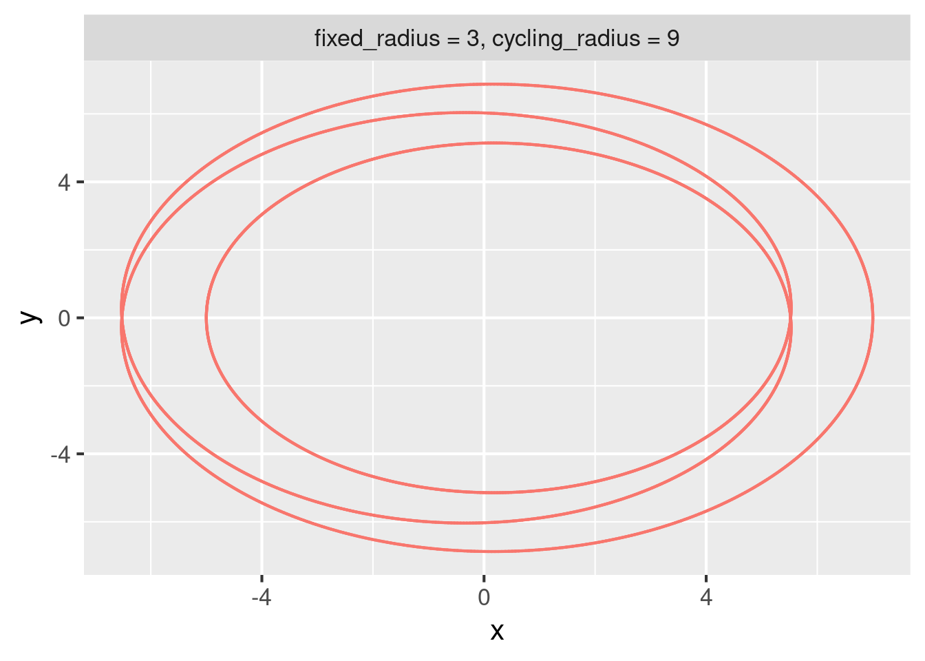

The tar_group_by() function in tarchetypes makes this branching easier. Using tar_group_by(), the pipeline condenses down to:

list(
  tar_group_by(
    points,
    bind_rows(
      spirograph_points(3, 9),
      spirograph_points(7, 2)
    ),
    fixed_radius,
    cycling_radius
  ),
  tar_target(
    single_plot,
    plot_spirographs(points),
    pattern = map(points),
    iteration = "list"
  )
)

For similar functions that branch across row groups, visit https://docs.ropensci.org/tarchetypes/reference/index.html#dynamic-grouped-data-frames.

15.8 Branching over files

Dynamic branching over files is tricky. A target with format = "file" treats the entire set of files as an irreducible bundle. That means in order to branch over files downstream, each file must already have its own branch. Here is a pipeline that begins with spirograph data files and loads each into a different dynamic branch.

# _targets.R
library(targets)
library(tarchetypes)
list(
  tar_target(paths, c("spirograph_dataset_1.csv", "spirograph_dataset_1.csv")),
  tar_target(files, paths, format = "file", pattern = map(paths)),
  tar_target(data, read_csv(files), pattern = map(files))
)

The tar_files() function from the tarchetypes package is shorthand for the first two targets above.

# _targets.R
library(targets)
library(tarchetypes)
list(
  tar_files(files, c("spirograph_dataset_1.csv", "spirograph_dataset_1.csv")),
  tar_target(data, read_csv(files), pattern = map(files))
)

15.9 Performance and batching

Dynamic branching makes it easy to create many targets. Unfortunately, if the number of targets exceeds several hundred thousand, overhead may build up and the package may slow down. Temporary workarounds can avoid overhead in specific cases: for example, the shortcut argument of tar_make(), and choosing a pattern like slice() or head() instead of a full map(). But to minimize overhead at scale, it is better to accomplish the same amount of work with a fewer number of targets. In other words, do more work inside each dynamic branch.

Batching is particularly useful to reduce overhead. In batching, each dynamic branch performs multiple computations instead of just one. The tarchetypes package supports several general-purpose functions that do batching automatically: most notably tar_rep() and tar_map_rep() for simulation studies and tar_group_count(), tar_group_size(), and tar_group_select() for batching over the rows of a data frame.

The packages in the R Targetopia support batching for specific use cases. For example, in stantargets, tar_stan_mcmc_rep_summary() dynamically branches over batches of simulated datasets for Stan models.

The targets-stan repository has an example of custom batching implemented from scratch. The goal of the pipeline is to validate a Bayesian model by simulating thousands of dataset, analyzing each with a Bayesian model, and assessing the overall accuracy of the inference. Rather than define a target for each dataset in model, the pipeline breaks up the work into batches, where each batch has multiple datasets or multiple analyses. Here is a version of the pipeline with 40 batches and 25 simulation reps per batch (1000 reps total in a pipeline of 82 targets).

# _targets.R
library(targets)
library(tarchetypes)
list(
  tar_target(model_file, compile_model("stan/model.stan"), format = "file"),
  tar_target(index_batch, seq_len(40)),
  tar_target(index_sim, seq_len(25)),
  tar_target(
    data_continuous,
    purrr::map_dfr(index_sim, ~simulate_data_continuous()),
    pattern = map(index_batch)
  ),
  tar_target(
    fit_continuous,
    map_sims(data_continuous, model_file = model_file),
    pattern = map(data_continuous)
  )
)

---

1. The pipeline uses code borrowed from the spiro package. The code in the spirograph_points() function is adapted from https://github.com/wjschne/spiro/blob/87f73ec37ceb0a7a9d09856ada8ae28d587a2ebd/R/spirograph.R under the CC0 1.0 Universal license: https://github.com/wjschne/spiro/blob/87f73ec37ceb0a7a9d09856ada8ae28d587a2ebd/LICENSE.md

2. See also https://books.ropensci.org/targets/debugging.html#workspaces.