Chapter 3 Walkthrough
A typical data analysis workflow is a sequence of data transformations. Raw data becomes tidy data, then turns into fitted models, summaries, and reports. Other analyses are usually variations of this pattern, and drake can easily accommodate them.
3.1 Set the stage.
To set up a project, load your packages,
library(drake)
library(dplyr)
library(ggplot2)
library(tidyr)
#>
#> Attaching package: 'tidyr'
#> The following objects are masked from 'package:drake':
#>
#>     expand, gather
load your custom functions,
create_plot <- function(data) {
  ggplot(data) +
    geom_histogram(aes(x = Ozone)) +
    theme_gray(24)
}
check any supporting files (optional),
## Get the files with drake_example("main").
file.exists("raw_data.xlsx")
#> [1] TRUE
file.exists("report.Rmd")
#> [1] TRUE
and plan what you are going to do.
plan <- drake_plan(
  raw_data = readxl::read_excel(file_in("raw_data.xlsx")),
  data = raw_data %>%
    mutate(Ozone = replace_na(Ozone, mean(Ozone, na.rm = TRUE))),
  hist = create_plot(data),
  fit = lm(Ozone ~ Wind + Temp, data),
  report = rmarkdown::render(
    knitr_in("report.Rmd"),
    output_file = file_out("report.html"),
    quiet = TRUE
  )
)

plan
#> # A tibble: 5 x 2
#>   target   command
#>   <chr>    <expr_lst>
#> 1 raw_data readxl::read_excel(file_in("raw_data.xlsx"))                        …
#> 2 data     raw_data %>% mutate(Ozone = replace_na(Ozone, mean(Ozone, na.rm = TR…
#> 3 hist     create_plot(data)                                                   …
#> 4 fit      lm(Ozone ~ Wind + Temp, data)                                       …
#> 5 report   rmarkdown::render(knitr_in("report.Rmd"), output_file = file_out("re…
Optionally, visualize your workflow to make sure you set it up correctly. The graph is interactive, so you can click, drag, hover, zoom, and explore.
vis_drake_graph(plan)3.2 Make your results.
So far, we have just been setting the stage. Use make() or r_make() to do the real work. Targets are built in the correct order regardless of the row order of plan.
make(plan) # See also r_make().
#> ▶ target raw_data
#> ▶ target data
#> ▶ target fit
#> ▶ target hist
#> ▶ target report
Except for output files like report.html, your output is stored in a hidden .drake/ folder. Reading it back is easy.
readd(data) %>% # See also loadd().
  head()
#> # A tibble: 6 x 6
#>   Ozone Solar.R  Wind  Temp Month   Day
#>   <dbl>   <dbl> <dbl> <dbl> <dbl> <dbl>
#> 1  41       190   7.4    67     5     1
#> 2  36       118   8      72     5     2
#> 3  12       149  12.6    74     5     3
#> 4  18       313  11.5    62     5     4
#> 5  42.1      NA  14.3    56     5     5
#> 6  28        NA  14.9    66     5     6
The graph shows everything up to date.
vis_drake_graph(plan) # See also r_vis_drake_graph().3.3 Go back and fix things.
You may look back on your work and see room for improvement, but it’s all good! The whole point of drake is to help you go back and change things quickly and painlessly. For example, we forgot to give our histogram a bin width.
readd(hist)
#> `stat_bin()` using `bins = 30`. Pick better value with `binwidth`.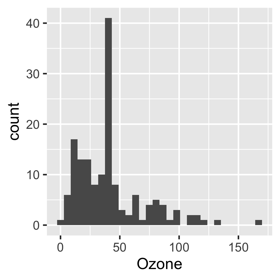
So let’s fix the plotting function.
create_plot <- function(data) {
  ggplot(data) +
    geom_histogram(aes(x = Ozone), binwidth = 10) +
    theme_gray(24)
}
drake knows which results are affected.
vis_drake_graph(plan) # See also r_vis_drake_graph().The next make() just builds hist and report. No point in wasting time on the data or model.
make(plan) # See also r_make().
#> ▶ target hist
#> ▶ target reportloadd(hist)
hist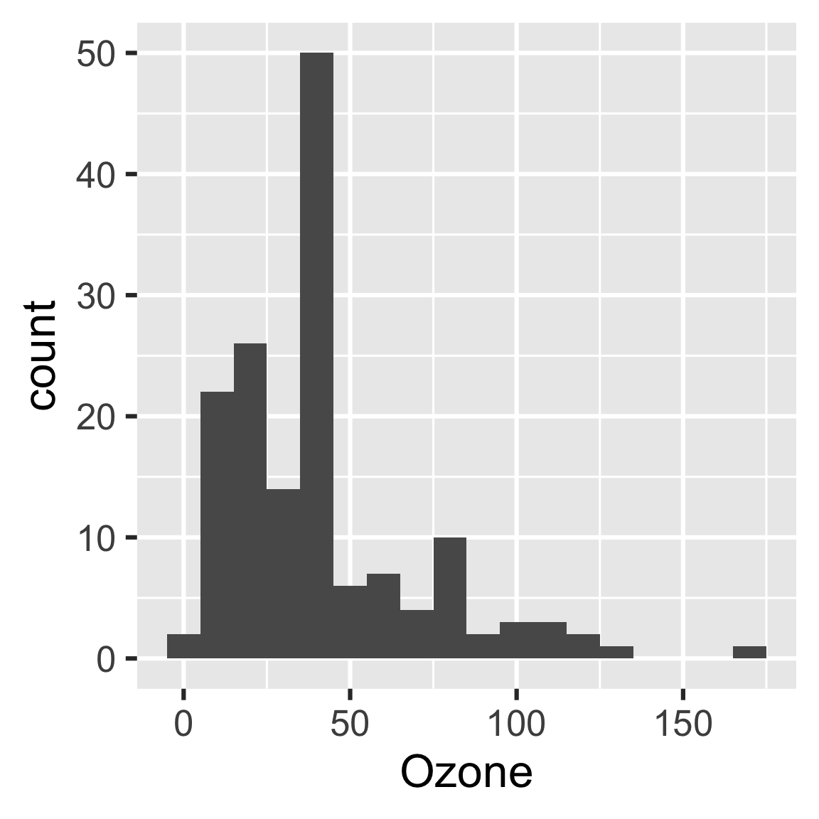
3.4 History and provenance
As of version 7.5.2, drake tracks the history and provenance of your targets:
what you built, when you built it, how you built it, the arguments you
used in your function calls, and how to get the data back.
history <- drake_history(analyze = TRUE)
history
#> # A tibble: 7 x 11
#>   target current built exists hash  command   seed runtime na.rm quiet
#>   <chr>  <lgl>   <chr> <lgl>  <chr> <chr>    <int>   <dbl> <lgl> <lgl>
#> 1 data   TRUE    2021… TRUE   11e2… "raw_d… 1.29e9 0.0200  TRUE  NA
#> 2 fit    TRUE    2021… TRUE   3c87… "lm(Oz… 1.11e9 0.003   NA    NA
#> 3 hist   FALSE   2021… TRUE   e100… "creat… 2.10e8 0.011   NA    NA
#> 4 hist   TRUE    2021… TRUE   4e36… "creat… 2.10e8 0.00400 NA    NA
#> 5 raw_d… TRUE    2021… TRUE   855d… "readx… 1.20e9 0.0130  NA    NA
#> 6 report TRUE    2021… TRUE   2454… "rmark… 1.30e9 1.52    NA    TRUE
#> 7 report TRUE    2021… TRUE   2454… "rmark… 1.30e9 0.885   NA    TRUE
#> # … with 1 more variable: output_file <chr>
Remarks:
- The
quietcolumn appears above because one of thedrake_plan()commands hasknit(quiet = TRUE). - The
hashcolumn identifies all the previous versions of your targets. As long asexistsisTRUE, you can recover old data. - Advanced: if you use
make(cache_log_file = TRUE)and put the cache log file under version control, you can match the hashes fromdrake_history()with thegitcommit history of your code.
Let’s use the history to recover the oldest histogram.
hash <- history %>%
  filter(target == "hist") %>%
  pull(hash) %>%
  head(n = 1)
cache <- drake_cache()
cache$get_value(hash)
#> `stat_bin()` using `bins = 30`. Pick better value with `binwidth`.
3.5 Reproducible data recovery and renaming
Remember how we made that change to our histogram? What if we want to change it back? If we revert create_plot(), make(plan, recover = TRUE) restores the original plot.
create_plot <- function(data) {
  ggplot(data) +
    geom_histogram(aes(x = Ozone)) +
    theme_gray(24)
}

# The report still needs to run in order to restore report.html.
make(plan, recover = TRUE)
#> ℹ unloading 1 targets from environment
#> ✔ recover hist
#> ▶ target report

readd(hist) # old histogram
#> `stat_bin()` using `bins = 30`. Pick better value with `binwidth`.
drake’s data recovery feature is another way to avoid rerunning commands. It is useful if:
- You want to revert to your old code, maybe with
git reset. - You accidentally
clean()ed a target and you want to get it back. - You want to rename an expensive target.
In version 7.5.2 and above, make(recover = TRUE) can salvage the values of old targets. Before building a target, drake checks if you have ever built something else with the same command, dependencies, seed, etc. that you have right now. If appropriate, drake assigns the old value to the new target instead of rerunning the command.
Caveats:
- This feature is still experimental.
- Recovery may not be a good idea if your external dependencies have changed a lot over time (R version, package environment, etc.).
3.5.1 Undoing clean()
# Is the data really gone?
clean() # garbage_collection = FALSE

# Nope!
make(plan, recover = TRUE) # The report still builds since report.md is gone.
#> ✔ recover raw_data
#> ✔ recover data
#> ✔ recover fit
#> ✔ recover hist
#> ✔ recover report

# When was the raw data *really* first built?
diagnose(raw_data)$date
#> [1] "2021-02-06 22:44:45.970593 +0000 GMT"
3.5.2 Renaming
You can use recovery to rename a target. The trick is to supply the random number generator seed that drake used with the old target name. Also, renaming a target unavoidably invalidates downstream targets.
# Get the old seed.
old_seed <- diagnose(data)$seed

# Now rename the data and supply the old seed.
plan <- drake_plan(
  raw_data = readxl::read_excel(file_in("raw_data.xlsx")),

  # Previously just named "data".
  airquality_data = target(
    raw_data %>%
      mutate(Ozone = replace_na(Ozone, mean(Ozone, na.rm = TRUE))),
    seed = !!old_seed
  ),

  # `airquality_data` will be recovered from `data`,
  # but `hist` and `fit` have changed commands,
  # so they will build from scratch.
  hist = create_plot(airquality_data),
  fit = lm(Ozone ~ Wind + Temp, airquality_data),
  report = rmarkdown::render(
    knitr_in("report.Rmd"),
    output_file = file_out("report.html"),
    quiet = TRUE
  )
)

make(plan, recover = TRUE)
#> ✔ recover airquality_data
#> ▶ target fit
#> ▶ target hist
#> ▶ target report
3.6 Try the code yourself!
Use drake_example("main") to download the code files for this example.
3.7 Thanks
Thanks to Kirill Müller for originally providing this example.