Chapter 9 Customer churn and deep learning
drake is designed for workflows with long runtimes, and a major use case is deep learning. This chapter demonstrates how to leverage drake to manage a deep learning workflow. The original example comes from a blog post by Matt Dancho, and the chapter’s content itself comes directly from this R notebook, part of an RStudio Solutions Engineering example demonstrating TensorFlow in R. The notebook is modified and redistributed under the terms of the Apache 2.0 license, copyright RStudio (details here).
9.1 Churn packages
First, we load our packages into a fresh R session.
library(drake)
library(keras)
library(tidyverse)
library(rsample)
library(recipes)
library(yardstick)
9.2 Churn functions
drake is R-focused and function-oriented. We create functions to preprocess the data,
prepare_recipe <- function(data) {
  data %>%
    training() %>%
    recipe(Churn ~ .) %>%
    step_rm(customerID) %>%
    step_naomit(all_outcomes(), all_predictors()) %>%
    step_discretize(tenure, options = list(cuts = 6)) %>%
    step_log(TotalCharges) %>%
    step_mutate(Churn = ifelse(Churn == "Yes", 1, 0)) %>%
    step_dummy(all_nominal(), -all_outcomes()) %>%
    step_center(all_predictors(), -all_outcomes()) %>%
    step_scale(all_predictors(), -all_outcomes()) %>%
    prep()
}
define a keras model, exposing arguments to set the dimensionality and activation functions of the layers,
define_model <- function(rec, units1, units2, act1, act2, act3) {
  input_shape <- ncol(
    juice(rec, all_predictors(), composition = "matrix")
  )
  keras_model_sequential() %>%
    layer_dense(
      units = units1,
      kernel_initializer = "uniform",
      activation = act1,
      input_shape = input_shape
    ) %>%
    layer_dropout(rate = 0.1) %>%
    layer_dense(
      units = units2,
      kernel_initializer = "uniform",
      activation = act2
    ) %>%
    layer_dropout(rate = 0.1) %>%
    layer_dense(
      units = 1,
      kernel_initializer = "uniform",
      activation = act3
    )
}
train a model,
train_model <- function(
  rec,
  units1 = 16,
  units2 = 16,
  act1 = "relu",
  act2 = "relu",
  act3 = "sigmoid"
) {
  model <- define_model(
    rec = rec,
    units1 = units1,
    units2 = units2,
    act1 = act1,
    act2 = act2,
    act3 = act3
  )
  compile(
    model,
    optimizer = "adam",
    loss = "binary_crossentropy",
    metrics = c("accuracy")
  )
  x_train_tbl <- juice(
    rec,
    all_predictors(),
    composition = "matrix"
  )
  y_train_vec <- juice(rec, all_outcomes()) %>%
    pull()
  fit(
    object = model,
    x = x_train_tbl,
    y = y_train_vec,
    batch_size = 32,
    epochs = 32,
    validation_split = 0.3,
    verbose = 0
  )
  model
}
compare predictions against reality,
confusion_matrix <- function(data, rec, model) {
  testing_data <- bake(rec, testing(data))
  x_test_tbl <- testing_data %>%
    select(-Churn) %>%
    as.matrix()
  y_test_vec <- testing_data %>%
    select(Churn) %>%
    pull()
  yhat_keras_class_vec <- model %>%
    predict_classes(x_test_tbl) %>%
    as.factor() %>%
    fct_recode(yes = "1", no = "0")
  yhat_keras_prob_vec <-
    model %>%
    predict_proba(x_test_tbl) %>%
    as.vector()
  test_truth <- y_test_vec %>%
    as.factor() %>%
    fct_recode(yes = "1", no = "0")
  estimates_keras_tbl <- tibble(
    truth = test_truth,
    estimate = yhat_keras_class_vec,
    class_prob = yhat_keras_prob_vec
  )
  estimates_keras_tbl %>%
    conf_mat(truth, estimate)
}
and compare the performance of multiple models.
compare_models <- function(...) {
  name <- match.call()[-1] %>%
    as.character()
  df <- map_df(list(...), summary) %>%
    filter(.metric %in% c("accuracy", "sens", "spec")) %>%
    mutate(name = rep(name, each = n() / length(name))) %>%
    rename(metric = .metric, estimate = .estimate)
  ggplot(df) +
    geom_line(aes(x = metric, y = estimate, color = name, group = name)) +
    theme_gray(24)
}
9.3 Churn plan
Next, we define our workflow in a drake plan. We will prepare the data, train different models with different activation functions, and compare the models in terms of performance.
activations <- c("relu", "sigmoid")

plan <- drake_plan(
  data = read_csv(file_in("customer_churn.csv"), col_types = cols()) %>%
    initial_split(prop = 0.3),
  rec = prepare_recipe(data),
  model = target(
    train_model(rec, act1 = act),
    format = "keras", # Supported in drake > 7.5.2 to store models properly.
    transform = map(act = !!activations)
  ),
  conf = target(
    confusion_matrix(data, rec, model),
    transform = map(model, .id = act)
  ),
  metrics = target(
    compare_models(conf),
    transform = combine(conf)
  )
)
The plan is a data frame with the steps we are going to do.
plan
#> # A tibble: 7 x 3
#>   target       command                                                    format
#>   <chr>        <expr_lst>                                                 <chr>
#> 1 conf_relu    confusion_matrix(data, rec, model_relu)                  … <NA>
#> 2 conf_sigmoid confusion_matrix(data, rec, model_sigmoid)               … <NA>
#> 3 data         read_csv(file_in("customer_churn.csv"), col_types = cols(… <NA>
#> 4 metrics      compare_models(conf_relu, conf_sigmoid)                  … <NA>
#> 5 model_relu   train_model(rec, act1 = "relu")                          … keras
#> 6 model_sigmo… train_model(rec, act1 = "sigmoid")                       … keras
#> 7 rec          prepare_recipe(data)                                     … <NA>
9.4 Churn dependency graph
The graph visualizes the dependency relationships among the steps of the workflow.
vis_drake_graph(plan)9.5 Run the Keras models
Call make() to actually run the workflow.
make(plan)
#> ▶ target data
#> ▶ target rec
#> ▶ target model_relu
#> ▶ target model_sigmoid
#> ▶ target conf_relu
#> ▶ target conf_sigmoid
#> ▶ target metrics
9.6 Inspect the Keras results
The two models performed about the same.
readd(metrics) # see also loadd()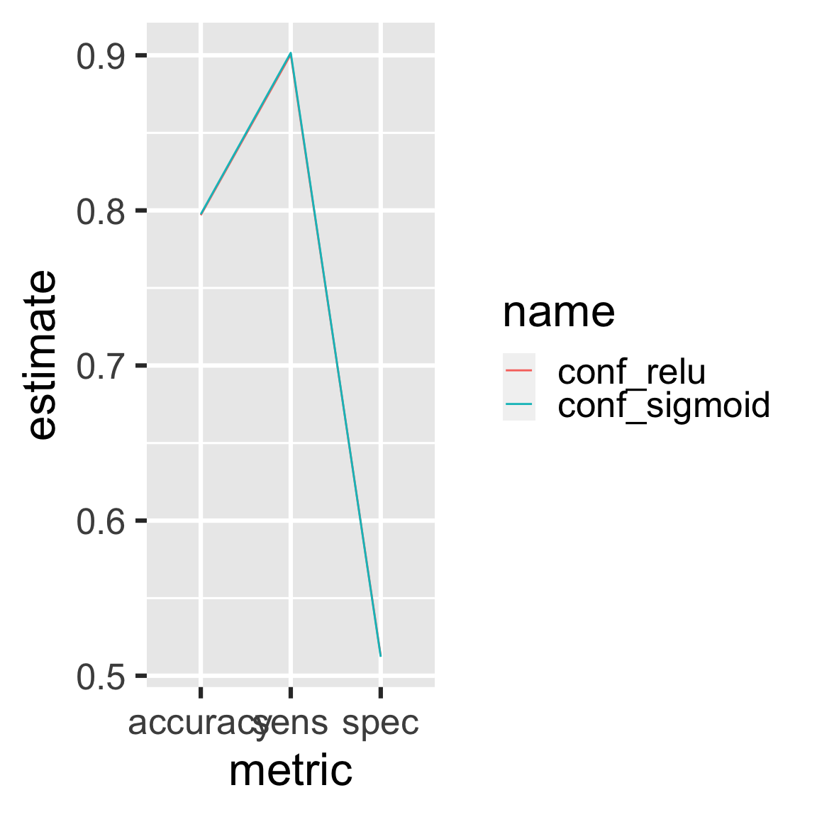
9.7 Add Keras models
Let’s try the softmax activation function.
activations <- c("relu", "sigmoid", "softmax")

plan <- drake_plan(
  data = read_csv(file_in("customer_churn.csv"), col_types = cols()) %>%
    initial_split(prop = 0.3),
  rec = prepare_recipe(data),
  model = target(
    train_model(rec, act1 = act),
    format = "keras", # Supported in drake > 7.5.2 to store models properly.
    transform = map(act = !!activations)
  ),
  conf = target(
    confusion_matrix(data, rec, model),
    transform = map(model, .id = act)
  ),
  metrics = target(
    compare_models(conf),
    transform = combine(conf)
  )
)vis_drake_graph(plan) # see also outdated() and predict_runtime()make() skips the relu and sigmoid models because they are already up to date. (Their dependencies did not change.) Only the softmax model needs to run.
make(plan)
#> ▶ target model_softmax
#> ▶ target conf_softmax
#> ▶ target metrics
9.8 Inspect the Churn results again
readd(metrics) # see also loadd()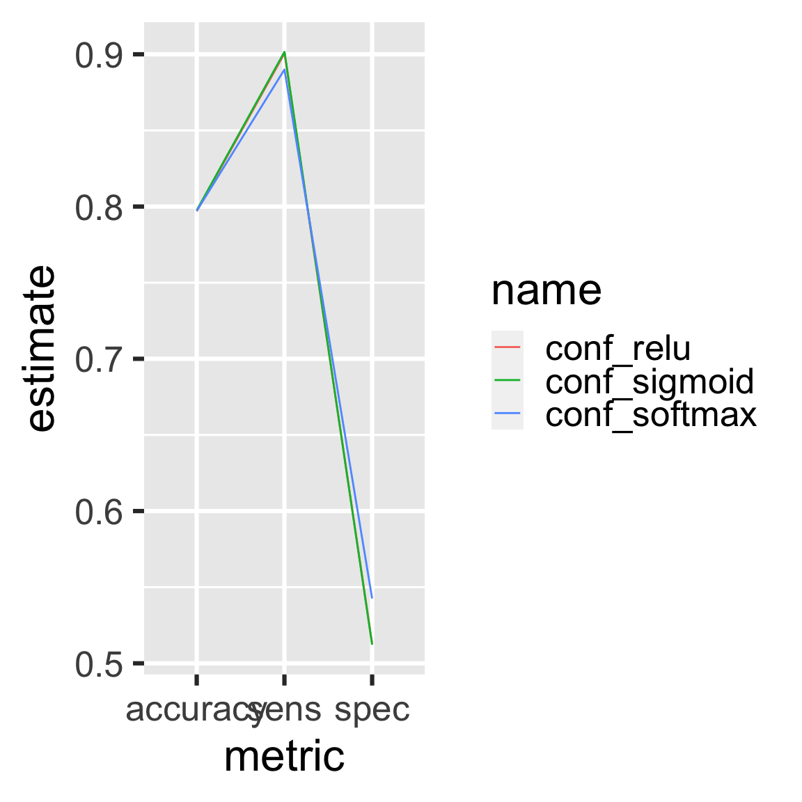
9.9 Update the Churn code
If you change upstream functions, even nested ones, drake automatically refits the affected models. Let’s increase dropout in both layers.
define_model <- function(rec, units1, units2, act1, act2, act3) {
  input_shape <- ncol(
    juice(rec, all_predictors(), composition = "matrix")
  )
  keras_model_sequential() %>%
    layer_dense(
      units = units1,
      kernel_initializer = "uniform",
      activation = act1,
      input_shape = input_shape
    ) %>%
    layer_dropout(rate = 0.15) %>% # Changed from 0.1 to 0.15.
    layer_dense(
      units = units2,
      kernel_initializer = "uniform",
      activation = act2
    ) %>%
    layer_dropout(rate = 0.15) %>% # Changed from 0.1 to 0.15.
    layer_dense(
      units = 1,
      kernel_initializer = "uniform",
      activation = act3
    )
}
All the models and downstream results are affected.
make(plan)
#> ▶ target model_relu
#> ▶ target model_sigmoid
#> ▶ target model_softmax
#> ▶ target conf_relu
#> ▶ target conf_sigmoid
#> ▶ target conf_softmax
#> ▶ target metrics
9.10 Churn history and provenance
drake tracks history and provenance. You can see which models you ran, when you ran them, how long they took, and which settings you tried (i.e. named arguments to function calls in your commands).
history <- drake_history()
history
#> # A tibble: 17 x 10
#>    target  current built    exists hash  command        seed runtime  prop act1
#>    <chr>   <lgl>   <chr>    <lgl>  <chr> <chr>         <int>   <dbl> <dbl> <chr>
#>  1 conf_r… FALSE   2021-02… TRUE   625c… "confusion_… 4.05e8   0.455  NA   <NA>
#>  2 conf_r… TRUE    2021-02… TRUE   0e43… "confusion_… 4.05e8   0.385  NA   <NA>
#>  3 conf_s… FALSE   2021-02… TRUE   6d39… "confusion_… 1.93e9   0.39   NA   <NA>
#>  4 conf_s… TRUE    2021-02… TRUE   edd4… "confusion_… 1.93e9   0.344  NA   <NA>
#>  5 conf_s… FALSE   2021-02… TRUE   6813… "confusion_… 1.80e9   0.370  NA   <NA>
#>  6 conf_s… TRUE    2021-02… TRUE   5079… "confusion_… 1.80e9   0.351  NA   <NA>
#>  7 data    TRUE    2021-02… TRUE   62d3… "read_csv(f… 1.29e9   0.085   0.3 <NA>
#>  8 metrics FALSE   2021-02… TRUE   00c6… "compare_mo… 1.21e9   0.053  NA   <NA>
#>  9 metrics FALSE   2021-02… TRUE   d3e7… "compare_mo… 1.21e9   0.075  NA   <NA>
#> 10 metrics TRUE    2021-02… TRUE   3a8e… "compare_mo… 1.21e9   0.061  NA   <NA>
#> 11 model_… FALSE   2021-02… TRUE   a52a… "train_mode… 1.47e9  10.2    NA   relu
#> 12 model_… TRUE    2021-02… TRUE   056b… "train_mode… 1.47e9   4.99   NA   relu
#> 13 model_… FALSE   2021-02… TRUE   8b5b… "train_mode… 1.26e9   4.93   NA   sigm…
#> 14 model_… TRUE    2021-02… TRUE   36e7… "train_mode… 1.26e9   5.02   NA   sigm…
#> 15 model_… FALSE   2021-02… TRUE   220e… "train_mode… 8.05e8   5.00   NA   soft…
#> 16 model_… TRUE    2021-02… TRUE   4e0c… "train_mode… 8.05e8   5.04   NA   soft…
#> 17 rec     TRUE    2021-02… TRUE   71f6… "prepare_re… 6.29e8   0.298  NA   <NA>
And as long as you did not run clean(garbage_collection = TRUE), you can get the old data back. Let’s find the oldest run of the relu model.
hash <- history %>%
  filter(act1 == "relu") %>%
  pull(hash) %>%
  head(n = 1)
drake_cache()$get_value(hash)
#> Model
#> Model: "sequential"
#> ________________________________________________________________________________
#> Layer (type)                        Output Shape                    Param #
#> ================================================================================
#> dense_2 (Dense)                     (None, 16)                      576
#> ________________________________________________________________________________
#> dropout_1 (Dropout)                 (None, 16)                      0
#> ________________________________________________________________________________
#> dense_1 (Dense)                     (None, 16)                      272
#> ________________________________________________________________________________
#> dropout (Dropout)                   (None, 16)                      0
#> ________________________________________________________________________________
#> dense (Dense)                       (None, 1)                       17
#> ================================================================================
#> Total params: 865
#> Trainable params: 865
#> Non-trainable params: 0
#> ________________________________________________________________________________